Tag: relativity

  • Mapping Music 12. FORM

    Rhythmic intensity is an important factor in shaping musical form. A former research project “Density Functions in the Structure of Modern Music” in the 1970s sought to quantify it along with several other core aspects of structure at play in shaping large-scale form.

    In the TIME chapters, we previously mentioned pace and showed how it can accelerate or decelerate in a line while tempo remains steady. (The Beethoven string quartet example Op. 135 illustrated that.) We have now also defined composite rhythm as an intersecting sum of rhythmic time points of lines, the layers of a textural fabric.

    Density

    In physical terms, density is a ratio comparing the amount of mass to the amount of space it takes up. Measuring time space, tempo (expressed in “M.M.” beats per minute) can convert a count of beats into a time-length in seconds:

    DURATION (in seconds) — multiply BEATS times 60, then divide by TEMPO

    Now we’re ready to measure the pace of a line for a bar or a whole phrase:

    PACE (Notes Per Second) — number of notes divided by the duration of the stream

    And then to quantify for a whole texture of rhythmic activity:

    RHYTHMIC DENSITY (Attack-Points Per Second) — number of note-starting time-points in the composite rhythm of the whole texture divided by the duration of the stream

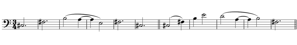
    Let’s go back to the Webern Symphonie Op. 21. Though called a symphony, it has only two movements. The second movement is a theme and variations with coda, each exactly 11 bars long in two-four meter. Here’s the theme:

    Op. 21, II — theme

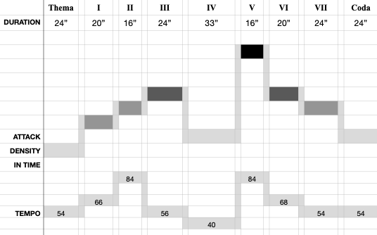
    Each variation, though 11 bars long like the theme, is in a different marked tempo. Each is distinguished by a contrasting degree of rhythmic density. And though the theme is a sparse (pointillistic) fabric, some variations are contrapuntally thick and intense.

    Rhythmic density and what we might define as textural density (how many lines woven into what octave span) basically trace the same unfolding through the variations. The exception is Variation V. There they diverge, intensely active rhythms but only three textural elements in a diffuse pitch span of almost four octaves.

    A graph of changing rhythmic density values in each variation highlights rhythmic density as the bolder line:

    density graph of Op. 21 II

    About broad form, this reveals that from the beginning, rhythmic density increases to a subordinate peak in Variation III and overall peak in Variation V, then variation by variation steps down to a coda that matches how we started with the sparse theme. In rhythmic density, the whole movement is an arch form, with Variation V the “climax.”

    In the first “abstract sound mobile” of my 2024 work, FOLIO, it is easier to hear changing density as the changing thickness of clouds of sound, swelling and subsiding.

    “Music of the Spheres”

    Relativity

    Modeling, the process of creating an overall design, can mean creating a new model or expanding the possibilities of an existing model. In Learning to Compose we identified and described three basic musical approaches:

    NARRATIVE MODELING — Designing by telling a story, with characters, themes, gestures, suspense. What will happen next?

    SPACIAL MODELING — Designing the size, shape, and texture of blocks or sections of material

    TEMPORAL MODELING — Designing the flow and momentum of events in the passing of perceived time

    Variation and contrast

    Contrast is the essential complement to developmental continuity in musical material, driving musical momentum. Theme and variations form is a straightforward, traditional example of narrative modeling balancing contrast and continuity. Each variation preserves some basic element of structure such as harmonic progression (or in the Webern example, the tone row). Each variation presents a setting of that theme element in distinctly different orchestration, texture, mode, tempo, or rhythmic character.

    The composer determines not just how and when to make a contrast, but how dramatic the contrast will be. Their fluctuations over time are the core of the composer’s instinctive variation skill. This is the impelling force that gives musical form a sense of going somewhere, of leading up to and flowing away from stable plateaus marking the structural pillars of large-scale form.

    FLUCTUATION — Magnitude of contrast from one moment or event to the next

    When analytically quantifying fluctuating data, the time scale of measurement matters. In avant-garde or experimental music, a stream of events may be high-contrast on the moment-to-moment scale but steady-state over broader time spans. Conversely and more traditionally, surface events may be continuous, while the bigger chunks of events, like one variation to the next, may pose more dramatic changes in parameters such as rhythmic density.

    In typical Beethoven or Brahms variations, material within each variation is continuous, not at all fluctuant. The contrast comes altogether in the next variation.

    That consideration plays out differently in Op. 21 II. There is the obvious contrast from one variation to the next; but within each variation, moment-to-moment surface continuity also fluctuates. Surface fluctuation in density factors occurs, especially from one 3-to-4-second “moment” to the next. (We can’t really call them phrases.)

    For the Op. 21 II. Theme and Variations, we can now say something deeper about changing rhythmic density as the variations progress. From the Theme through the first two variations, rhythmic density increases gradually to Variation III. But then the fluctuation of rhythmic density spikes, dropping significantly for Variation IV, then suddenly increasing to its highest level in Variation V.

    large-scale time form

    It is not only Variation V’s greatest rhythmic intensity but also dramatically increased roller-coaster fluctuation, dropping then surging, that makes Variation V the climax of the movement. 

    Macro-structure

    Though Webern may not have thought consciously about Schwankung (fluctuation), this is how composers manipulate momentum to make a climax and shape large-scale form. Likewise, approaching a final ending, not only do fluctuations typically diminish, but also rate of change subsides — the overall change factor levels out to zero. These are examples of temporal modeling.

    The parameters of a musical event are numerous, a multidimensional matrix of at least six distinct, interacting qualities: each sound event’s loudness, resonance, timbre or sound color, duration, pitch (frequency), and time point of initiation. Imagine this as a six-dimensional space. In fact, physicists have imagined the structure of matter as exhibiting many more than six dimensions in string theory, M theory, etc.

    Musical structure establishes the relativity of these parameters, though not exactly the way Einstein explained time, space, gravity, and energy with mathematical precision. Some structures such as the Schoenberg Farben example relate constellation harmony to sound color. Threnody relates rhythmic activity to fabrics of sound in a broad pitch space (spatial modeling). Counterpoint balances rhythmic relationships, metric placement of lines, and synchronicity with their intervallic relationships of consonance and dissonance. Ostinato music manipulates phase relationships.

    And, as observed in Part I, temporal density, the rapidity of fluctuations and larger contrasts in these structures, propels our experience of the whole in time.

    In Thinking in Numbers, Daniel Tammet wrote about a mathematical study of poetry,

    “The best poems . . . combined in equal parts the predictability of meter with the novelty of unusual words. Too much meter made a poem banal; too much freewheeling . . . rendered it hard to follow. The delicate balance of convention and invention gives meaning to what we say.”

    The essence of music’s large-scale temporal form is the relativity of overlapping, fluctuating musical structures in time, repeating, contrasting, interrupting, truncating, expanding, certainly recurring, or simply evolving. Designing a large-scale musical form combines temporal modeling, narrative modeling, and spatial modeling — a pacing plan, a storytelling rhetoric, an architecture of interrelated components. 

    Coda

    sound mass . . . sound color . . . pitch constellations

    ostinato repetition . . . changing density

    evolving form . . . cosmic time

    In Become Ocean (2013), John Luther Adams takes a deep dive into a serene sound sea, incorporating all of the elements and structures we have explored in our mapping journey.

    John Luther Adams – Become Ocean (2013)

    . . . and we have just begun gazing into

    the vast space of color and complexity

    in the Music Universe . . .

    © 2026 – All Rights Reserved

    Thomas S. Clark

    Continue reading Mapping the Music Universe . . .

    MapLab 1. Generate a Gymnopédie

    TClarkArtMusic.com

  • Mapping Music 9. LINE

    Think about levels of structure scientists study in our universe.

    They dive deep into atomic structure, below electrons spinning around a nucleus of protons and neutrons, discovering subatomic particles like the meson and boson. At the other extreme, they gather observations to speculate about the shape of the entire expanding universe. We understand the structure of our planet, of our solar system, and our Milky Way galaxy.

    “We are slowed down sound and light waves,

    a walking bundle of frequencies tuned into the cosmos.”

    — Albert Einstein

    Think about how artists build structures that establish a style  . . .

    Painting engages techniques to create texture, rising to broad descriptions of style that actually describe structure: impressionism, cubism, pointillism. Musically, macro-structure is thought of as texture and form. Texture has been treated in broad descriptive categories: monody, homophony, polyphony, counterpoint, and more recently, sound mass, each focusing on the number of distinct parts, voices, or layers and how they interrelate.

    Structure and Relativity

    Shrinking our metaphor from the vastness of the universe down to the physical immediacy of cloth . . .

    A woven fabric has a longitudinal warp and a perpendicular crossing weft. Part II explored the vertical-pitch “weft” of harmonic design. Now we return to the “warp” in music, longitudinal time streams of events. In keeping with our standard conception of time as horizontal and pitch as vertical, let’s name each longitudinal “warp” element:

    LINE — an element of a musical fabric consisting of a conforming stream in time of similar events (notes, pitches, colors, drum sounds, etc.)

    Now we can go back to “monody, homophony, polyphony” and at least identify how many lines are in a musical fabric, from one (monody) to many (polyphony). But to distinguish between homophony with its matching, rhythmically aligned lines from polyphony with its more diverse set of lines of different nature, we must distinguish different types of lines to determine the extent to which the lines of a polyphonic fabric “match.”

    There are limitless number of combinations of characters for a line and thus an infinite number of fabrics possible. We will stick to six parameters and simple observational characterizations for each parameter. Since we are swimming in the painting and weaving metaphors, we will color-code these six parameters. Each parameter will be distinguished with just two binary descriptors, a simpler or purer character or a more intense or complex character in that parameter.

    distinguishing parameters

    Since there are 7 parameters and two possible descriptors for each parameter, the total number of permutations is 2 to the 7th power = 128 possible combinations. That means, however, if there are two lines in the fabric, the number of possible combinations rises to 16,384 — plenty of choice for creative composing. And with 4 lines, the number of possible combinations explodes to more than 268 billion!

    More simply, with these defined characteristics we can redefine “homophony” to mean more than one line that match characteristics, and typically are in rhythmic alignment (synchronized). Indeed, most musical fabrics involve quite a bit of similarity between multiple lines. In a typical traditional “melody-and-accompaniment” fabric, there are only three distinct lines, melody, bass line, and chords, even if the chords are actually in two or more matching instrumental or vocal parts.

    The following example is taken from the Allegretto movement of Beethoven’s String Quartet Op. 135.

    String Quartet Op. 135 Allegretto, mm. 25-48

    In the first two bars of this example from Op. 135, there are actually only two lines in the fabric, the melody (1st violin) and repeated chord tones (the other three instruments aligned in 16th-notes) — common homophony.

     Op. 135 violin vs. other lines

    Though there is no dynamic marking for the 1st violin, it will be played as a prominent line, what Schoenberg would have called the Hauptstimme. By the third bar of the second system (11th bar of the example), there are three lines, violins / viola / cello, and by the next bar, briefly, all four instruments have distinct fabric threads. By the end of the excerpt, all parts have joined in homophonic unity.

    Melodic shape

    Melodic connotes a singable tune of primary focus; here it is meant simply as any line of successive single pitches. In the general descriptors of texture, we referred to smooth and angular shape. Let’s be more precise. First, there is the general size of melodic intervals. As music practice moved from Medieval/Renaissance through 18th-Century styles, smaller intervals, steps and small skips predominated. 19th-Century styles introduced a greater proportion of larger “leaping” intervals, 6ths, 7ths, 9ths. And those large, disjunct intervals became the norm for much 20th-Cenury music.

    Another important melodic shape factor is directional.

    TURN — a melodic note is approached in one direction (up or down) and left in the opposite direction

    Some turns are trivial and do not complicate melodic shape, such as trills and back-and-forth oscillations.

    turns in Elegy line

    The first phrase, starting on Eb, goes up to E then down to D — turning on the middle note, E. The next two phrases are increasingly complex in shape.

    Elegy 2nd and 3rd phrases

    The phrase starting on the lower B rises to G# then turns down on that G# to A, then back up from A, and finally back down, turning on Bb. There are three turning points, G#, A, and Bb, in a phrase of only six pitches and five melodic intervals. Combined with the fact that each melodic interval is a different size (9 s.t., 3, 8, 1, 3) except the last (reusing the downward 3 semitone interval), this is a rather complex, angular shape.

    The third phrase, starting on the higher B, is even more complex in angular shape: turns on every pitch except the C# — that is five turns in just 7 melodic intervals between 8 pitches.

    A side note of analytic math:

    • Number of pitches (#P) minus 1 = number of melodic intervals
    • Number of melodic intervals minus 1 = number of “opportunities” for the line to turn (#P – 2)
    • Shape complexity = #T / (#P – 2) ranging from zero to 1

    Pitch recurrence

    RETRACING — melodic line returning within a phrase to the same pitch (in the same octave) as previously sounded in the phrase

    Distinguished from a pitch being repeated (immediately), a retracing is a recurrence after other intervening pitches. It contributes to structural stability in the phase, a sense of staying in one place. Conversely, when retracings are avoided in the shape of the line, the sense is more of progressing, even of wandering, as in the Elegy example above. (Use of a 12-tone row to construct a line is a way to methodically avoid retracing any pitch until all 12 pitch classes have been introduced.)

    Back to Bartók — two orchestral lines studied in the Pitch chapter. The first example (from the opening fugue of Music for Strings, Percussion and Celeste) is scored for viola, but here I show it in bass clef for those a bit challenged by alto clef.

    fugue subject

    Mapping the line on a time/pitch graph for analysis, the first phrase avoids any retracing. The next three phrases make only one retracing each: back to Bb in the second phrase (highlighted in blue); back to C# in the third (in red); retracing back to C in the fourth (in green). (There are fainter retracings back to the previous phrase in each not shown.)

    The second is a low string line from the opening of Concerto for Orchestra.

    Concerto for Orchestra retracings

    In this example, both phrases are built with two retracings, C# and F# in the first phrase, F# and B in the second phrase.

    In this manner, retracing of pitches builds the support structure for the architecture of many lines.

    © 2026 – All Rights Reserved

    Thomas S. Clark

    Continue reading Mapping the Music Universe:

    TClarkArtMusic.com 

  • Mapping Music — PRELUDE

    The heavenly motions are nothing

    but a continuous song for several voices,

    perceived not by the ear but by the intellect,

    music that sets landmarks

    in the immeasurable flow of time.”

    Galileo

    When we gaze at stars and planets, they appear as stationary points of light, fixed in place in what seems a random pattern across the entire night sky visible to our hemisphere. Time stands still.

    Throughout human time, humans have imagined that stars make picture patterns we name as constellations: fish, warriors, goddesses, animals. Only the persistent observers, such as astronomers, identify their nightly march across the sky, rising in the east and disappearing below the western horizon.

    Metaphor

    Musical sounds mark points in time, like stars. They form immediately into recognizable patterns we call chords, melodies, rhythms, memorable themes. They convey a sense of motion, time surging forward or slackening in our perception of their well choreographed parade.

    Astronomers observing and mapping (recording) the myriad points discovered that some of the stars are actually whole galaxies, with exotic forms of spirals and clouds. They observed through the color of the light that all these objects are racing away from us and each other in an expanding universe.

    Mapping music means cataloging many possible patterns, distinguishing their contrasts and commonalities. We will explore how to measure and compare the periodic rhythmic streams of musical events and their changing momentum. We will define and employ a simple but powerful math tool for cataloging and then creatively sculpting with all natures of harmony and melodic line in our 88-key chromatic universe. We will explore how master composers weave colorful fabrics and grand structures from skillfully crafted materials.

    Pursuing periodicity

    My music-mapping Periodicity Project began in 2021 as a comprehensive catalog of musical patterns and processes, meant to provide simple tools for understanding the complexities of modern music. It grew into this book, Mapping the Music Universe, written for anyone who is curious about how music works, especially in the 20th-21st-century modern and “post-modern” eras. For me as a composer, it is also an exploration of how some less traveled conceptual paths lead to interesting creative possibilities.

    In 1989 I co-authored a conceptually ground-breaking composition textbook with Larry Austin, Learning to Compose: Modes, Materials, and Models of Musical Invention. My next book, ARRAYS, was an aural skills workbook covering basic modal, tonal, and “post-tonal” music of the Renaissance through the Twentieth Century. Mapping the Music Universe draws in part on the ideas and approaches of both these now out-of-print publications.

    A common assumption within Western culture is that Science is all about observation, measurement, precision, and mathematical rigor . . . and Art is all about the “i” words: imagination, inspiration, intuition, improvisation. Science is Deductive, art is Creative. Our culture has begun to recognize the commonality of all these intellectual strengths, that the best Science can be creatively intuitive and great Art can be rigorous.

    Pioneer map makers

    As an educated musician and professional composer, I also have long been deeply interested in science, especially astronomy. Having read a great deal of general science writing, I am inspired particularly by ground-breaking pioneers who methodically and comprehensively mapped the possibilities of their particular field.

    Johann Joseph Fux — wrote Gradus ad Parnassum in 1725, codifying basic contrapuntal principles of Renaissance music.

    William Smith — a rural surveyor, in 1799 drew a colorful map of the subterranean rock strata of his county in English coal country, launching the modern science of geology.   

    Meriwether Lewis — kept extensive journals of the 1804-1806 Lewis and Clark Expedition, documenting and illustrating the discovered new world of the Northwest.  

    Dmitri Mendeleev — devised a “periodic table of the chemical elements,” published in 1869, providing a solid basis for modern chemistry through its graphic and organizational genius.

    Amédée Mouchez — launched an ambitious international star-mapping project (Carte du Ciel) in 1887 at the Paris Observatory.

    Henrietta Swan Leavitt — worked at the Harvard College Observatory as a “computer,” examining thousands of photographic plates from telescopes to measure and catalog the brightness of stars, identified 1777 variable stars.

    Lawrence Herbert — invented the Pantone system in 1956 to systematize color for printing ink and fabrics.

    Allen Forte — published an article in 1964 that launched musical set theory, defining, classifying and comparing all possible collections of “pitch classes” drawn from the equal-tempered 12-tone chromatic galaxy.

    The work and insights of the two on the list representing rigorous study of music, Fux and Forte, were part of my formal education in music and later an integral part of my teaching of composition and music theory.

    Maps

    Carte du Ciel was an ambitious second phase of an international star-mapping project initiated in 1887 by Paris Observatory director Amédée Mouchez.  A new photographic process revolutionizing the gathering of telescope images inspired the first phase, the Astrographic Catalogue of a dense, whole-sky array of star positions. Carte du Ciel, never completed after 70 years, used the Catalogue as a reference system for a complex survey of the vast field of even fainter images.

    Celebrating the grand metaphor relating astronomy to art music, here is my 8-minute computer-music sound sculpture. In the music, ghostly wisps of sound are punctuated by brighter bursts, clustered in a natural, not-quite randomly dispersed texture.

    _______________

    Looking ahead

    The blog-post chapters of Mapping the Music Universe will proceed in three broad phases, progressing logically from fundamental — time and periodicity — to pitch space, then to larger structures, texture and form. Within each phase, various topics are presented in a progressive order, but jumping in at any point is fine.

    Terms will sometimes be freshly coined. Graphic figures will include notated musical examples, tables, and graphic illustrations of patterns and their relationships. Big Ideas — Periodicity, Complexity, Symmetry, Relativity — will be explored using precise mathematical arrays as well as broad metaphors. Newly composed sample etudes will illustrate aurally.

    Along the way, “Map Labs” will present step-by-step recipes to compose simple pieces based on models of different compositional genres. Each Lab includes an original sample piece following the Map Lab guidelines, illustrating one possible creative outcome.

    Welcome! Join this creative journey of discovery . . .

    a composer’s expedition.

    © 2026 – All Rights Reserved

    Thomas S. Clark

    Continue reading Mapping the Music Universe:

    1. TIME

    TClarkArtMusic.com